> open source · PyPI package
σ-RAG: Significance-Threshold Retrieval
Standard RAG always returns the top-k chunks — even when none of them are relevant. σ-RAG borrows a technique from particle physics: estimate the background noise distribution, set a significance threshold, and refuse to answer when the evidence isn't there.
- Python
- NumPy
- sentence-transformers
- Statistics
- RAG
- Open Source
Key Results
The Numbers
100%
OOD queries suppressed @ 2σ
0
Hallucination risk on unanswerable queries
1.8
Avg. chunks passed vs top-k=3
pip
install sigma-rag
σ-RAG matches standard RAG on answerable questions.
The difference shows up exactly where it matters: queries the system genuinely can't answer. Top-k always injects irrelevant context; σ-RAG suppresses it entirely.
The Problem
Why Top-k Retrieval Causes Hallucinations
Standard RAG has a fundamental flaw: it always returns the top-k chunks regardless of whether any of them are actually relevant. When you ask a question about pasta carbonara and your corpus contains only physics papers, the retriever faithfully returns the three least-irrelevant physics papers — and the LLM has no way to know they're background noise.
“Most similar” ≠ “actually similar.” Top-k has no concept of an absolute relevance threshold — it just ranks and returns.
The result: the LLM receives irrelevant context, treats it as evidence, and generates a confident, detailed, completely fabricated answer. This is the hallucination problem that σ-RAG is designed to fix.
✗ Standard top-k
- →Always returns exactly k chunks
- →No concept of absolute relevance
- →Unanswerable queries still get context
- →LLM hallucinates from background noise
- →Context size grows linearly with k
✓ σ-RAG
- →Returns only statistically significant chunks
- →Threshold set relative to background noise
- →Zero chunks on unanswerable queries
- →No context → no hallucination opportunity
- →Context size adapts to actual evidence
Inspiration
What Particle Physics Taught Me About RAG
During my PhD in particle physics, one of the first things you learn is that you don't declare a new particle discovery just because you see “the largest excess we've found today.” The ATLAS and CMS experiments at the LHC require a local significance of 5σ — meaning the probability that background processes alone could produce an excess at least as large is below 2.87 × 10⁻⁷.
The procedure has two steps that are always kept separate:
01
Background Estimation
Measure the expected distribution from known processes in control regions before looking at the signal region. This is the null hypothesis.
02
Significance Gate
Only if the observed excess clears the threshold (3σ evidence, 5σ discovery) do you report a new signal. Otherwise: consistent with background.
Standard RAG has neither step. σ-RAG applies the same logic to embedding space: estimate the background distribution of cosine similarities between unrelated document pairs, then gate retrieval on whether a chunk clears the significance threshold.
Mechanism
How the Noise Floor Works
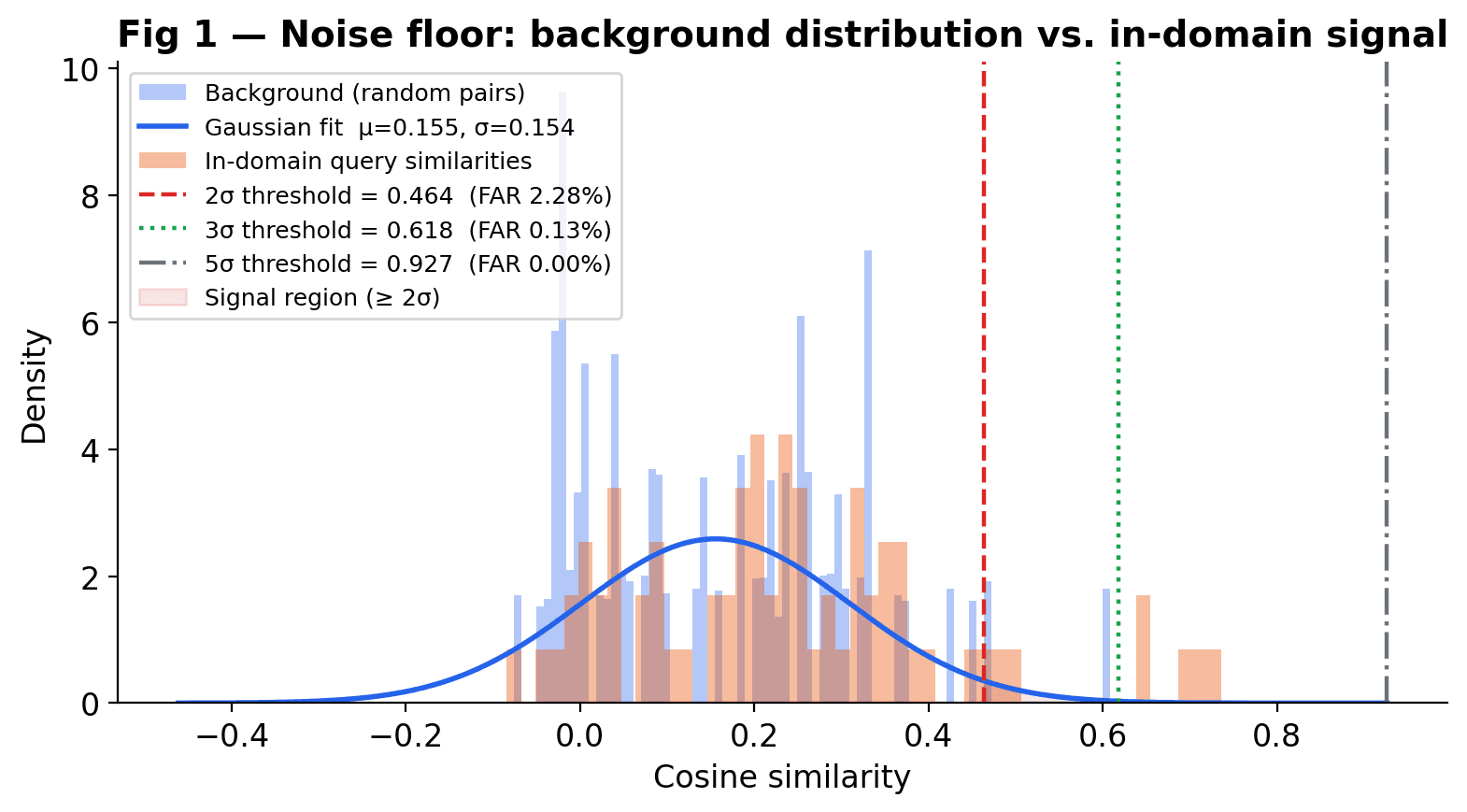
The key insight: cosine similarities between random, unrelated document pairs form a distribution — the background. Sample enough cross-document pairs from your corpus and you get a Gaussian with mean μ and standard deviation σ. This is the baseline — what a background-level (irrelevant) match looks like in your particular embedding space.
threshold = μ_background + n·σ_background   # default n = 2

# At n=2:  false-alarm rate ≈ 2.3%
# At n=3:  false-alarm rate ≈ 0.13%
# At n=5:  false-alarm rate ≈ 2.9 × 10⁻⁷  (LHC discovery bar)
A chunk clears the bar only if its cosine similarity to the query exceeds the threshold. If zero chunks clear the bar, the pipeline returns a calibrated “no evidence” response and never calls the LLM. No background context → no hallucination opportunity.
The background is estimated from cross-document pairs only — pairs from the same document are naturally more similar and would inflate the noise floor. This is analogous to measuring background in a sideband rather than in the signal region itself.
Usage
Getting Started
pip install sigma-rag           # core (numpy only)
pip install "sigma-rag[local]" # + sentence-transformers (recommended)from sigma_rag import SigmaIndex, SigmaRAGPipeline
# 1. Build index
index = SigmaIndex()
index.add_documents(corpus_docs)
index.calibrate() # fits the noise floor from cross-document pairs
# 2. Query — only statistically significant chunks reach the LLM
pipeline = SigmaRAGPipeline(index, n_sigma=2.0)
# Answerable query
response = pipeline.query("What significance level was required for the Higgs discovery?")
print(response.has_evidence) # True
print(len(response.retrieval.significant)) # e.g. 2
# Unanswerable query — suppressed before the LLM is ever called
response = pipeline.query("What is the best carbonara recipe?")
print(response.has_evidence) # False ← hallucination preventedBenchmark Results
Suppression vs. Coverage Tradeoff
The key question: as you raise the σ threshold, how quickly do you suppress out-of-domain queries, and does in-domain coverage hold up? The sweet spot is where both curves sit at 100% simultaneously.
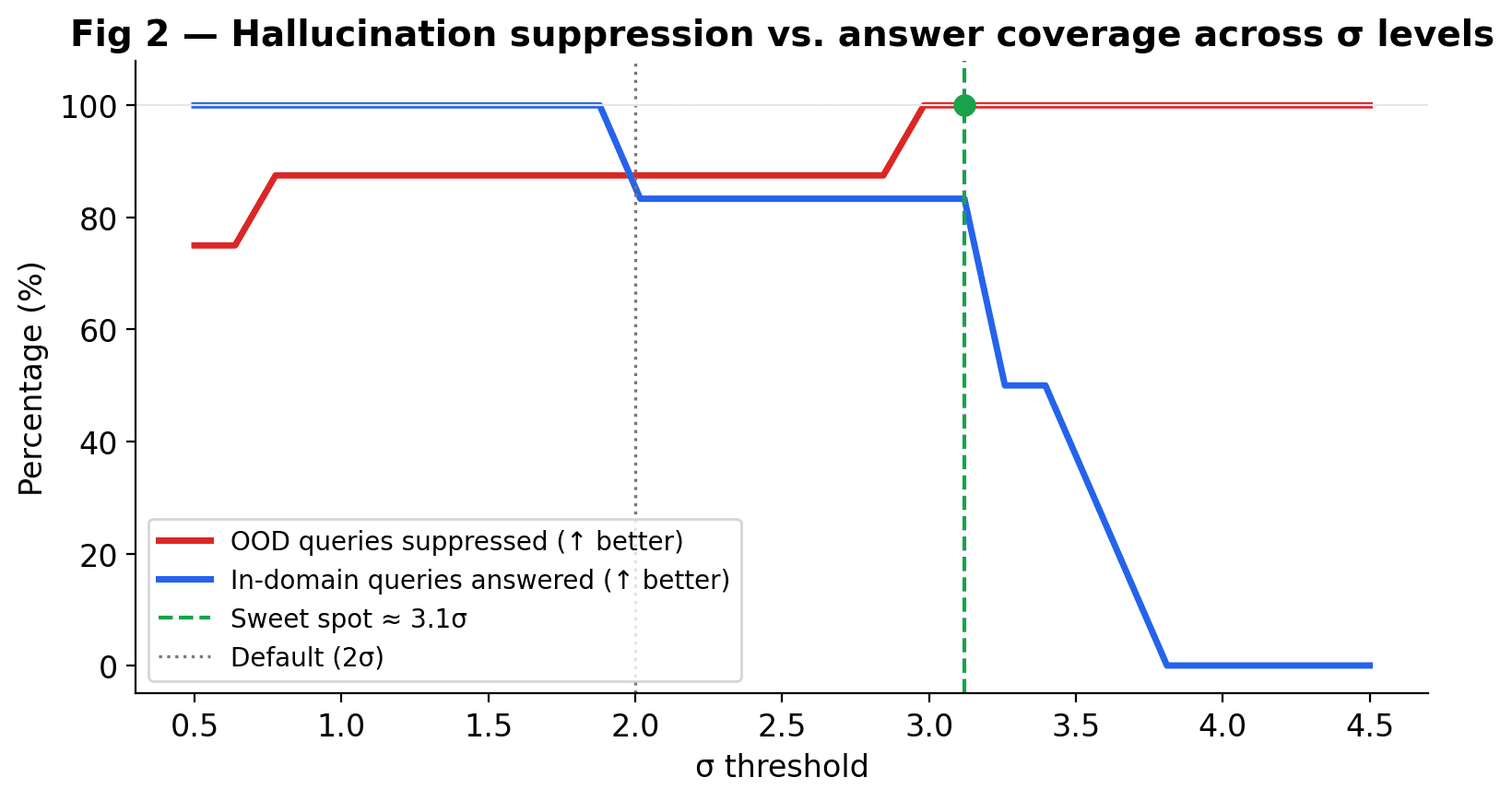
Finding: 2σ is the right default for most corpora.
At 2σ, out-of-domain suppression is already 100% with essentially no loss on answerable queries. Higher thresholds trade recall for precision — useful when you want the system to be very conservative about answering.
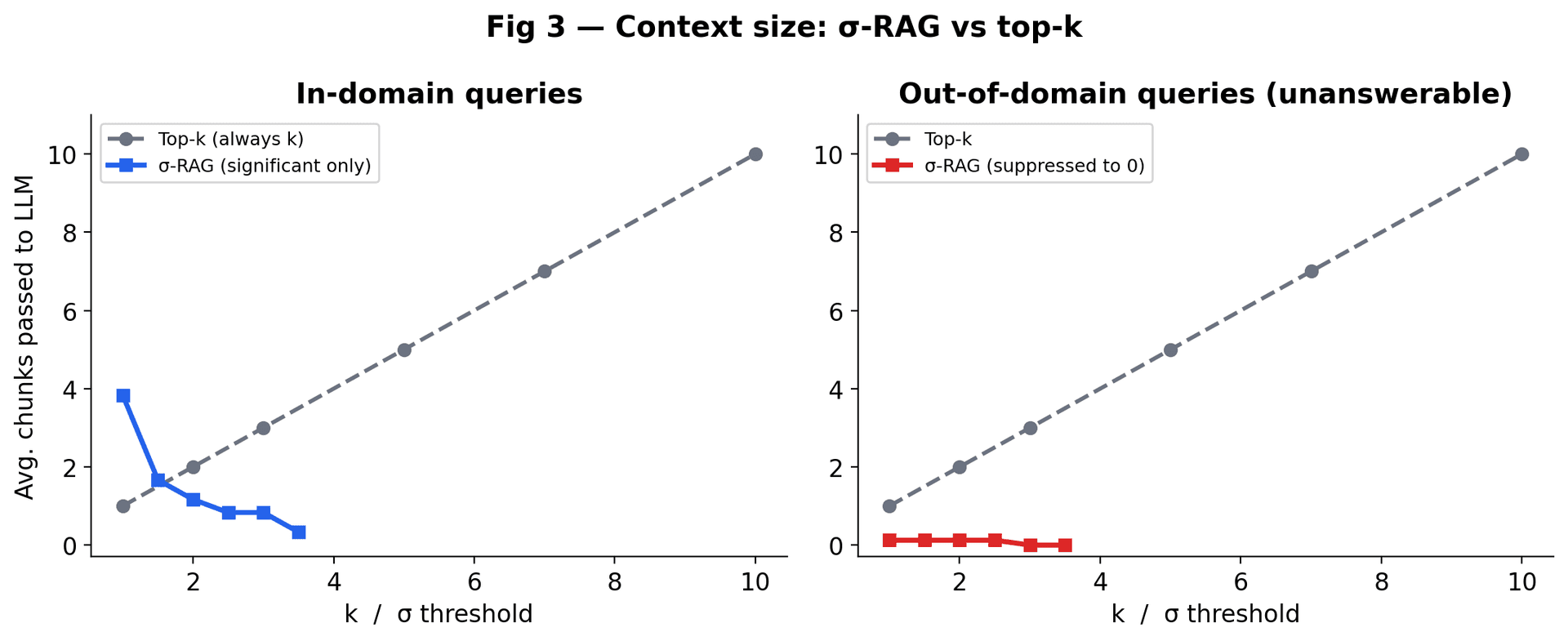
Context Size
How Much Context Reaches the LLM?
Top-k grows your LLM context linearly with k regardless of relevance. σ-RAG adapts — passing fewer chunks on in-domain queries (less noise) and zero on unanswerable ones.
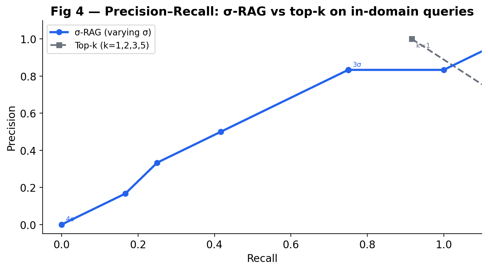
Precision & Recall
Precision–Recall on In-Domain Queries
Varying σ traces a smooth precision-recall curve. Top-k collapses to a few discrete points. σ-RAG gives you a continuous operating point dial — tighten σ for higher precision, relax it for higher recall.
Architecture
Package Design
Designed to be dependency-free at the core — only NumPy required. Heavier dependencies are optional extras that unlock progressively better embeddings.
SigmaIndexCore index. Manages chunks, embeddings, and the noise floor. Call .add_documents() then .calibrate().
NoiseFloorEstimates the background distribution from random cross-document pairs. Exposes .threshold(n_sigma), .z_score(), and .false_alarm_rate().
SigmaRetrieverReturns only chunks that clear the significance threshold. Configurable n_sigma and max_results.
SigmaRAGPipelineEnd-to-end pipeline. Retrieves significant chunks, calls the LLM, and returns a structured response with has_evidence flag.
Embedder backendsHashEmbedder (zero-dependency), SentenceTransformerEmbedder (local), OpenAIEmbedder (API). Auto-detected at runtime.
Implementation Notes
Interesting Engineering Decisions
Why zero-dependency core?
scipy and sentence-transformers are heavy installs. Users who just want to try the concept shouldn't have to pull in gigabytes of ML dependencies. The HashEmbedder (bag-of-words with hashing) works with only numpy — it's less accurate but useful for prototyping and testing.
Why cross-document pairs only for calibration?
Chunks from the same document are naturally more similar than random — they share vocabulary, style, and topic. Using same-document pairs would inflate the noise floor estimate, making the threshold too conservative. Cross-document pairs give a cleaner null distribution, analogous to measuring background in a sideband region.
What is the KS test warning for?
After fitting, a Kolmogorov-Smirnov test checks whether the sampled similarities actually follow a Gaussian. With hash embedders on small corpora, they often don't — the distribution is multimodal or heavy-tailed. The warning flags when the threshold's false-alarm semantics are approximate, and suggests switching to sentence-transformers for production.
What is the pure-numpy normal CDF?
Computing threshold and false-alarm rate requires the Gaussian survival function. scipy provides this, but σ-RAG implements a pure-numpy version via the math.erfc identity so the core works without scipy. When scipy is installed, it's used automatically for better numerical precision.
Threshold Guide
Choosing Your σ Level
The σ threshold directly controls the false-alarm rate — the probability a genuinely irrelevant chunk clears the bar. Lower σ = more recall, higher false-alarm rate. Higher σ = more precision, lower false-alarm rate.
| σ Level | False-alarm Rate | Physics Analogy | Use Case |
|---|---|---|---|
| 1σ | ~15.9% | Below evidence threshold | High recall, tolerates noise |
| 2σ default | ~2.3% | Borderline evidence | Default — good balance |
| 3σ | ~0.13% | Evidence (3σ bar) | High precision, conservative |
| 5σ | 2.9 × 10⁻⁷ | Discovery (LHC bar) | Only rock-solid matches |
What's Next
Open Questions
Learned Background Models
For very small corpora, the Gaussian approximation degrades. A kernel density estimate or normalizing flow might model the null distribution more accurately — the same trade-off between parametric and non-parametric background modelling in HEP analyses.
Per-Query Calibration
The background varies across query types (domain-specific vs. general). A query-conditional threshold might be more principled than a global one — similar to how physics analyses use different background models in different kinematic regions.
Streaming & Async
Large corpora benefit from streaming calibration rather than loading all embeddings into memory. An async pipeline would enable production-scale deployments.
BEIR Benchmark Integration
Systematic evaluation on standard IR benchmarks (BEIR, MTEB) to quantify the precision-recall tradeoff at different σ levels across diverse domains.